What is a Search Algorithm?
Moving from one place to another is a task that we humans do almost every day. We try to find the shortest path with the help of A * Search (Heuristic Search) that enables us to reach our destinations faster and make the whole process of travelling as efficient as possible. In the old days, we would trial and error with the paths available and had to assume which path taken was shorter or longer.
Now, we have algorithms that can help us find the shortest paths virtually. We just need to add costs (time, money etc.) to the graphs or maps and the algorithm finds us the path that we need to take to reach our destination as quick as possible. Many algorithms were developed through the years for this problem and A* is one the most popular algorithms out there.
Tree search Algorithm
A tree structure is a hierarchy of linked nodes where each node represents a particular state. Nodes have none, one or more child nodes. A solution is a path from the “root” node to a “goal” node. Tree search algorithms attempt to find a solution by traversing the tree structure – starting at the root node and examining the child nodes in a systematic way.
Tree search algorithms differ by the order in which nodes are traversed and can be classified into two main groups:
- Blind search algorithms (e.g. “Breadth-first” and “Depth-first”) use a fixed strategy to methodically traverse the search tree. Blind search is not suitable for complex problems as the the large search space makes them impractical given time and memory constraints.
- Best-first search algorithms (e.g. “Greedy” and “A*”) use a heuristic function to determine the order in which nodes are traversed, giving preference to states that are judged to be most likely to reach the required goal. Using a “heuristic” search strategy reduces the search space to a more manageable size.
A search strategy is complete if it is guaranteed to find a solution if one exists. A search strategy is optimal if it is guaranteed to find the best solution when several solutions exists.
Breadth-First Search
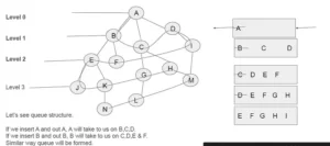
It starts from the root node, explores the neighboring nodes first and moves towards the next level neighbors. It generates one tree at a time until the solution is found. It can be implemented using FIFO queue data structure. This method provides shortest path to the solution.
If branching factor (average number of child nodes for a given node) = b and depth = d,
then number of nodes at level d = bd. The total no of nodes created in worst case is b + b2 + b3 + … + bd.
Disadvantage − Since each level of nodes is saved for creating next one, it consumes a lot of memory space. Space requirement to store nodes is exponential.
Its complexity depends on the number of nodes. It can check duplicate nodes.

Depth-First Search
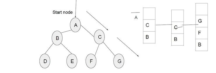
It is implemented in recursion with LIFO stack data structure. It creates the same set of nodes as Breadth-First method, only in the different order.
As the nodes on the single path are stored in each iteration from root to leaf node, the space requirement to store nodes is linear. With branching factor b and depth as m, the storage space is bm.
Disadvantage − This algorithm may not terminate and go on infinitely on one path. The solution to this issue is to choose a cut-off depth. If the ideal cut-off is d, and if chosen cut-off is lesser than d, then this algorithm may fail. If chosen cut-off is more than d, then execution time increases.
Its complexity depends on the number of paths. It cannot check duplicate nodes.

Bidirectional Search
It searches forward from initial state and backward from goal state till both meet to identify a common state.
The path from initial state is concatenated with the inverse path from the goal state. Each search is done only up to half of the total path.
Uniform Cost Search
Sorting is done in increasing cost of the path to a node. It always expands the least cost node. It is identical to Breadth First search if each transition has the same cost.
It explores paths in the increasing order of cost.
Disadvantage − There can be multiple long paths with the cost ≤ C*. Uniform Cost search must explore them all.
Iterative Deepening Depth-First Search
It performs depth-first search to level 1, starts over, executes a complete depth-first search to level 2, and continues in such way till the solution is found.
It never creates a node until all lower nodes are generated. It only saves a stack of nodes. The algorithm ends when it finds a solution at depth d. The number of nodes created at depth d is bd and at depth d-1 is bd-1
Heuristic Search
To solve large problems with large number of possible states, problem-specific knowledge needs to be added to increase the efficiency of search algorithms.
Heuristic Evaluation Functions
They calculate the cost of optimal path between two states. A heuristic function for sliding-tiles games is computed by counting number of moves that each tile makes from its goal state and adding these number of moves for all tiles.
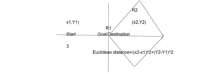
There are different methods to calculate the Heuristic value. Euclidean distance is one of them. It is also called a straight-line method. If we calculate distance we will R1 is the right optimal path to follow.

Manhattan distance
Manhattan distance is another method to calculate an optimal path. Let’s understand this by the 8-Puzzle problem.
Let’s calculate the Manhattan distance from a start position to a goal position. If you see ‘1’ is on the same position in goal
state so we do not have to move vertically or horizontally so distance will be zero. Look at ‘2’ in the goal state, we have to
move one step left movement will be one. Similarly, we calculate manhattan distance for all states by moving the number in
start state and chooses the state which has less manhattan value.

Pure Heuristic Search
It expands nodes in the order of their heuristic values. It creates two lists, a closed list for the already expanded nodes and an open list for the created but unexpanded nodes.
In each iteration, a node with a minimum heuristic value is expanded, all its child nodes are created and placed in the closed list. Then, the heuristic function is applied to the child nodes and they are placed in the open list according to their heuristic value. The shorter paths are saved and the longer ones are disposed.
A * Search
(What is heuristic function in ai, What is heuristic search in ai)
What exactly is the A* algorithm? It is an advanced BFS algorithm that searches for shorter paths first rather than the longer paths. A* is optimal as well as a complete algorithm.
Optimal meaning that A* is sure to find the least cost from the source to the destination and Complete meaning that it is going to find all the paths that are available to us from the source to the destination.
So that makes A* the best algorithm right? Well, in most cases, yes. But A* is slow and also the space it requires is a lot as it saves all the possible paths that are available to us. This makes other faster algorithms have an upper hand over A* but it is nevertheless, one of the best algorithms out there.
Formula
F = G + H
F – F is the parameter of A* which is the sum of the other parameters G and H and is the least cost from one node to the next node. This parameter is responsible for helping us find the most optimal path from our source to destination.
- G – G is the cost of moving from one node to the other node. This parameter changes for every node as we move up to find the most optimal path.
- H – H is the heuristic/estimated path between the current code to the destination node. This cost is not actual but is, in reality, a guess cost that we use to find which could be the most optimal path between our source and destination.
A * Search Explanation
Consider a square grid having many obstacles and we are given a starting cell and a target cell. We want to reach the target cell from the starting cell as quickly as possible. Here A* Search Algorithm comes to the rescue.
What A* Search Algorithm? does is that at each step it picks the node according to a value-‘Ff’ which is a parameter equal to the sum of two other parameters – ‘G’ and ‘H’. At each step it picks the node/cell having the lowest ‘F’, and process that node/cell.
We define ‘G’ and ‘H’ as simply as possible below
G = the movement cost to move from the starting point to a given square on the grid, following the path generated to get there.
H = the estimated movement cost to move from that given square on the grid to the final destination. This is often referred to as the heuristic, which is nothing but a kind of smart guess. We really don’t know the actual distance until we find the path, because all sorts of things can be in the way (walls, water, etc.).
Let’s understand A* search technique with an example.
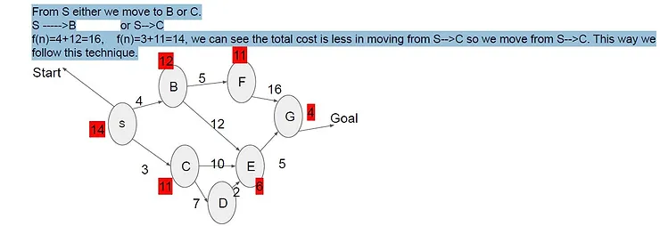
The values marked in red are estimated values or heuristic value. We find this value with help of BFS technique. Lets we
want to go to start node (S) to goal node (G), the other node like B,F,C,E and D are the n nodes. The cost to reach from S
node to B node is 4 similarly for other node is given. Let’s calculate cost.
f(n)=g(n)+h(n)
f(S) = 0+14=14
From S either we move to B or C.
S —–>B or S–>C
f(n)=4+12=16, f(n)=3+11=14, we can see the total cost is less in moving from S–>C so we move from S–>C. This way we
follow this technique.

A * Search Algorithm
- Add start node to list
- For all the neighbouring nodes, find the least cost F node
- Switch to the closed list
- For 8 nodes adjacent to the current node
- If the node is not reachable, ignore it. Else
- If the node is not on the open list, move it to the open list and calculate f, g, h.
- If the node is on the open list, check if the path it offers is less than the current path and change to it if it does so.
- Stop working when
- You find the destination
- You cannot find the destination going through all possible points
Pseudo-Code of the Algorithm
1. let the openList equal empty list of nodes
2. let the closedList equal empty list of nodes
3. put the startNode on the openList (leave it's f at zero)
4. while the openList is not empty
5.                    let the currentNode equal the node with the least f value
6.                    remove the currentNode from the openList
7.                    add the currentNode to the closedList
8.                    if currentNode is the goal10.
9.                           You've found the end!
10.                 let the children of the currentNode equal the adjacent nodes
11.                  for each child in the children
12.                         if child is in the closedList
13.                               continue to beginning of for loop
14.                         child.g = currentNode.g + distance between child and current
15.                        child.h = distance from child to end
16.                        child.f = child.g + child.h
17.                        if child.position is in the openList's nodes positions
18.                            if the child.g is higher than the openList node's g
19.                                        continue to beginning of for loop
20.                            add the child to the openList
Read more